ml-a03-polynomial

import numpy as np
import matplotlib.pyplot as plt
from sklearn.preprocessing import PolynomialFeatures
from sklearn.linear_model import LinearRegression

data = np.genfromtxt("job.csv", delimiter=",")
x_data = data[1:,1]
y_data = data[1:,2]
plt.scatter(x_data,y_data)
plt.show()

# In this example, we use the linearRegression, we can see that the line does not match well the points

x_data = data[1:,1,np.newaxis]
y_data = data[1:,2,np.newaxis]
model = LinearRegression()
model.fit(x_data, y_data)

plt.plot(x_data,y_data, 'b.')
plt.plot(x_data,model.predict(x_data), 'r')
plt.show()

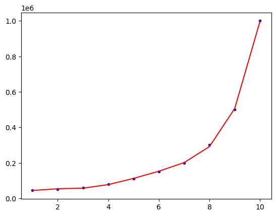
poly_reg = PolynomialFeatures(degree=5)
# Polynomial is used to add the features to the data, degree=1 => add data * power 0, degree = 2 => add data * power 0 and data * power 1
x_poly = poly_reg.fit_transform(x_data)
lin_reg = LinearRegression()
lin_reg.fit(x_poly, y_data)

x_poly

array([[1.0000e+00, 1.0000e+00, 1.0000e+00, 1.0000e+00, 1.0000e+00,
        1.0000e+00],
       [1.0000e+00, 2.0000e+00, 4.0000e+00, 8.0000e+00, 1.6000e+01,
        3.2000e+01],
       [1.0000e+00, 3.0000e+00, 9.0000e+00, 2.7000e+01, 8.1000e+01,
        2.4300e+02],
       [1.0000e+00, 4.0000e+00, 1.6000e+01, 6.4000e+01, 2.5600e+02,
        1.0240e+03],
       [1.0000e+00, 5.0000e+00, 2.5000e+01, 1.2500e+02, 6.2500e+02,
        3.1250e+03],
       [1.0000e+00, 6.0000e+00, 3.6000e+01, 2.1600e+02, 1.2960e+03,
        7.7760e+03],
       [1.0000e+00, 7.0000e+00, 4.9000e+01, 3.4300e+02, 2.4010e+03,
        1.6807e+04],
       [1.0000e+00, 8.0000e+00, 6.4000e+01, 5.1200e+02, 4.0960e+03,
        3.2768e+04],
       [1.0000e+00, 9.0000e+00, 8.1000e+01, 7.2900e+02, 6.5610e+03,
        5.9049e+04],
       [1.0000e+00, 1.0000e+01, 1.0000e+02, 1.0000e+03, 1.0000e+04,
        1.0000e+05]])

plt.plot(x_data, y_data, 'b.')
plt.plot(x_data, lin_reg.predict(x_poly), 'r')
plt.show()

PS:
job.csv